14 KiB
title, subtitle, author, license, affiliation, abstract, date, papersize, fontsize, documentclass, margin, slideNumber
| title | subtitle | author | license | affiliation | abstract | date | papersize | fontsize | documentclass | margin | slideNumber |
|---|---|---|---|---|---|---|---|---|---|---|---|
| Chemodiversity | A short overview of this project | Stefan Dresselhaus | BSD | Theoretic Biology Group<br> Bielefeld University | Attempt to find indications for chemodiversity in the plant secondary metabolism according to the screening hypothesis | \today | a4 | 10pt | scrartcl | 0.2 | true |
- It was observed, that many plants seem to produce many compounds with no obvious purpose
- Using resources to produce such compounds (instead of i.e. growing) should yield a fitness-disadvantage
- one expects evolution to eliminate such behavior
Question: Why is this behavior observed?
- Are these compounds necessary for some unresearched reason?
- unknown environmental effects?
- unknown intermediate products for necessary defenses?
- speculative diversity because they could be useful after genetic mutations?
Screening Hypothesis
- First suggested by Jones & Firn (1991)
- new (random) compounds are rarely biologically active
- plants have a higher chance finding an active compound if they diversify
- many (inactive) compounds are sustained for a while because they may be precursors to biologically active substances
. . .
There are indications for and against this hypothesis by various groups.
Setting up a simulation
If you wish to make apple pie from scratch, you must first create the universe
- Carl Sagan
Defining Chemistry
- First of all we define the chemistry of our environment, so we know all possible interactions and can manipulate them at will.
- We differentiate between
Substrate{.haskell} andProducts{.haskell}:Substrate{.haskell } can just be used (i.e. real substrates if the whole metabolism should be simulated,PPM{.haskell}^[1]^ in our simplified case)Products{.haskell } are nodes in our chemistry environment.
- In Code:
data Compound = Substrate Nutrient
              | Produced Component
              | GenericCompound Int
::: footer ^[1]^: plants primary metabolism :::
Usage in the current Model
- The Model used for evaluation just has one
Substrate{.haskell}:
PPM{.haskell} with a fixed Amount to account for effects of sucking primary-metabolism-products out of the primary metabolic cycle - This is used to simulate i.e. worse growth, fertility and other things affecting the fitness of a plant.
- We are not using named Compounds, but restrict to generic
Compound 1{.haskell},Compound 2{.haskell} ... - Not done, but worth exploring:
- Take a "real-world" snapshot of Nutrients and Compounds and recreate them
- See if the simulation follows the real world
Defining a Metabolism
-
We define
Enzyme{.haskell}s as- having a recipe for a chemical reaction
- are reversible
- may have dependencies on catalysts to be present
- may have higher dominance over other enzymes with the same reaction
-
Input can be
Substrate{.haskell} and/orProducts{.haskell} -
Outputs can only be
Products{.haskell} -
\RightarrowThis makes them to Edges in a graph combining the chemical compounds
Usage in the current Model
Enzyme{.haskell}s all- only map
1{.haskell} input to1{.haskell} Output with a production rate of1{.haskell} perEnzyme{.haskell}
(i.e.-1 Compound 2 -> +1 Compound 5{.haskell}) - are equally dominant
- need no catalysts
- only map
Defining Predators
Predator{.haskell}s consist of- a list of
Compound{.haskell}s that can kill them - a fitness impact (
[0..1]) as the probability of killing the plant - an expected number of attacks per generation
- a probability (
[0..1]) of appearing in a single generation
- a list of
Predator{.haskell} need not necessary be biologically motivated- i.e. rare, nearly devastating attacks (floods, droughts, ...) with realistic probabilities
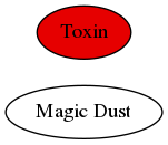
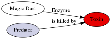
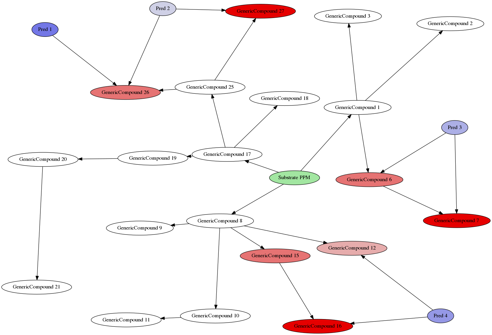
Example Environment
:::::::::::::: {.columns}
::: {.column width=37%}
- The complete environment now consists of
:::
::: {.column width=63% .fragment}
Additional rules:
- Every "subtree" from the marked
PPM{.haskell} is treated as a separate species (fungi, animals, ...)
\RightarrowEvery predator can only be affected by toxins in the same part of the tree - Trees can be automatically generated in a decent manner to search for environmens where specific effects may arise :::
::::::::::::::
::::: notes :::::
CTRL+Click for zoom!
- All starts at PPM (Plant Primary Metabolism)
- Red = Toxic
- Blue = Predators
::::
Plants
A Plant{.haskell} consists of
- a
Genome{.haskell}, a simple list of genes- Triple of
(Enzyme, Quantity, Activation){.haskell} - without order or locality (i.e. interference of neighboring genes)
Quantity{.haskell} is just an optimization (=Int) to group identicalActivation{.haskell}sActivation{.haskell} is a float\in [0..1]to regulate the activity of theEnzyme{.haskell} genetically
- Triple of
- an
absorbNutrients{.haskell}-Function to simulate various effects when absorbing nutrients out of the environment, depending on the environment (i.e. can use informations about chemistry, predators, etc.)- Not used in our simulation, as we only have
PPM{.haskell} as "nutrient" and we take everything given to us.
- Not used in our simulation, as we only have
Metabolism simulation
Creation of compounds from the given resources is an iterative process:
-
First of all we create a conversion Matrix
\Delta_cwith corresponding startvectors_0. -
We now iterate
s_i = (\mathbb{1} + \Delta_c) \cdot s_{i-1}for a fixed number of times (currently:100) to simulate the metabolism^[2]^.::: footer ::: ^[2]^: Thats a 'lie', we calculate
(\mathbb{1} + \Delta_c)^{100}efficiently vialapack-internals ::: -
Entries in the matrix come from the
Genome{.haskell}: anEnzyme{.haskell} which convertsitojwith quantityqand activityayield $$\begin{eqnarray*} \Delta_c[i,j] &\mathrel{+}=& q\cdot a,\ \Delta_c[j,i] &\mathrel{+}=& q\cdot a, \ \Delta_c[i,i] &\mathrel{-}=& q\cdot a, \ \Delta_c[j,j] &\mathrel{-}=& q\cdot a \end{eqnarray*}.$$- This makes the Enzyme-reaction invertible as both ways get treated equally.
Metabolism-example
-
Given a simple Metabolism with
1nutrient (first row/column) and2Enzymes in sequence, we have given\Delta_cwtih corresponding startvectors_0: $$\Delta_c = 0.01 \cdot \begin{pmatrix} -1 & 1 & 0 \ 1 & -2 & 1 \ 0 & 1 & -1 \ \end{pmatrix}, s_0 = \begin{pmatrix}\text{PPM:} & 3 \ \text{Compound1:} & 0 \ \text{Compound2:} & 0\end{pmatrix}.$$ -
In the simulation this yields us
s_{100} \approx \begin{pmatrix}\text{PPM:} & 1 \\ \text{Compound1:} & 1 \\ \text{Compound2:} & 1\end{pmatrix},which is the expected outcome for an equilibrium.
Assumptions for metabolism simulation
- All Enzymes are there from the beginning
- All Enzyme-reactions are reversible without loss
- static conversion-matrix for fast calculations (unsuited, if i.e. enzymes depend on catalysts)
- One genetic enzyme corresponds to (infinitely) many real (proportional weaker) enzymes in the plant, which get controlled via the "activation" parameter
Fitness
- We handle fitness as
\text{survival-probability} \in [0..1]and model each detrimental effect as probability which get multiplied together. - To calculate the fitness of an individual we take three distinct effects into
consideration:
- Static costs of enzymes
- Creating enzymes weakens the primary cycle and thus possibly beneficial
traits (growth, attraction of beneficial organisms, ...)
F_s := \text{static_cost_factor} \cdot \sum_i q_i \cdot a_i \quad | \quad (e_i,q_i, a_i) \in \text{Genome} - limits the amount of dormant enzymes
- Creating enzymes weakens the primary cycle and thus possibly beneficial
traits (growth, attraction of beneficial organisms, ...)
- Cost of active enzymes
- Cost of using up nutrients
F_e := \text{active_cost_factor} \cdot \frac{\text{Nutrients used}}{\text{Nutrients available}}
- Cost of using up nutrients
- Deterrence of attackers
F_d(next slide)
- Static costs of enzymes
Attacker
-
Predators are modeled after Svennungsen et al. (2007)
-
Each predator has an expected number of attacks
P_a, that are poisson-distributed with impactP_i. -
Plants can defend themselves via
- toxins that the predator is affected by with impact-probability
D_t(P_i) - herd-immunity via effects like automimicry:
D_{pop} = \mathbb{E}[D_t(P_i)]
- toxins that the predator is affected by with impact-probability
-
All this yields the formula:
F_d := 1 - e^{- (D_{pop} \cdot P_a) (1-D_t(P_i))} -
The attacker-model is only valid for many reasonable assumptions
- equilibrium population dynamics
- equal dense population
- which individual to attack is independently chosen
- etc. (Details in the paper linked above)
Haploid mating
-
We hold the population-size fixed at
100 -
Each plant has a reproduction-probability of
p(\textrm{reproduction}) = \frac{\textrm{plant-fitness}}{\textrm{total fitness in population}}yielding a fitness-weighted distribution from that
100new offspring are drawn -
in inheritance each gene of the parent goes through different steps (with given default-values)^[3]^
::::: footer ^[3]^: in case of quantity
q > 1the process is repeatedqtimes independently. ::::- mutation: with
p_{mut} = 0.01another random enzyme is produced, but activation kept - duplication: with
p_{dup} = 0.05the gene gets duplicated (quantity+1) - deletion: with
p_{del} = p_{dup}the gene get deleted (or quantity-1) - addition: with
p_{add} = 0.005an additional gene producing a random enzyme with activation0.5gets added as mutation from genes we do not track (i.e. primary cycle) - activation-noise: activation is changed by
c_{noise} = \pm 0.01drawn from a uniform distribution, clamped to[0..1]
- mutation: with
:::: notes
- Default values not motivated in any way!
- finding out how these values influence is core! ::::
Simulations
- Overall question: What parameters are necessary for chemodiversity?
- How can we see chemodiversity?
- We define an Enzyme
Eas divers, if the average of this Enzyme in the population stays below0.5, soE_i \in E_{div} \text{iff.} \mathbb{E}[E_i] < 0.5 - We can then count the number of diverse Enzymes per plant $E_{d,p_i} = |\left\lbrace E_i | E_i \in E_{div}, E_{i,p_i} > 0.5, \right\rbrace|$
- To get an insight into how this behaves we observe several other parameters
every generation:
- Fitness
\in [0..1] - Number of different compounds created
- Amount of compounds created
- Number of Plants theoretically resistant to predator
i(i.e. can produce a toxin to defend themselves, albeit not to100\%.
- Fitness
Simulations (cont.)
- General setup of the simulation:
- All using the example-environment shown before
27different compounds,1Nutrient (simulating the primary metabolism)7of27compounds are toxic- at least
3compounds are needed for total immunity 4predators set toAlwaysAttack{.haskell}
- Duration of
2000generations \text{static_enzyme_cost} = 0.02\text{nutrient_impact} = 0.1
- All using the example-environment shown before
- Different setups tested:
- Behavior of predators (
AlwaysAttack{.haskell},AttackRandom{.haskell},AttackInterval 10{.haskell},AttackInterval 100{.haskell}) - varying
\text{static_enzyme_cost}from0.0to0.20in steps of0.02- effectively limits the amount of maximal enzymes to
\frac{1}{\text{static_enzyme_cost}}
- effectively limits the amount of maximal enzymes to
- varying
\text{nutrient_impact}from0.0to1.0in steps of0.1- makes toxins less/more costly to produce
- Behavior of predators (
Results
It doesn't matter how beautiful your theory is, it doesn't matter how smart you are. If it doesn't agree with experiment, it's wrong.
- Richard P. Feynman


