---
title: Evaluation of the Performance of Randomized FFD Control Grids
subtitle: Master Thesis
author: Stefan Dresselhaus
affiliation: Graphics & Geometry Group
...
# Introduction
- Many modern industrial design processes require advanced optimization methods
due to increased complexity
- Examples are
- physical domains
- aerodynamics (i.e. drag)
- fluid dynamics (i.e. throughput of liquid)
- NP-hard problems
- layouting of circuit boards
- stacking of 3D--objects
-----
# Motivation
- Evolutionary algorithms cope especially well with these problem domains
- But formulation can be tricky
-----
# Motivation
- Problems tend to be very complex
- i.e. a surface with $n$ vertices has $3\cdot n$ Degrees of Freedom (DoF).
- Need for a small-dimensional representation that manipulates the
high-dimensional problem-space.
- We concentrate on smooth deformations ($C^3$-continuous)
- But what representation is good?
-----
# What representation is good?
- In biological evolution this measure is called *evolvability*.
- no consensus on definition
- meaning varies from context to context
- measurable?
- Measure depends on representation as well.
-----
# RBF and FFD
- Andreas Richter uses Radial Basis Functions (RBF) to smoothly deform meshes
-----
# RBF and FFD
- My master thesis transferred his idea to Freeform-Deformation (FFD)
- same setup
- same measurements
- same results?

-----
# Outline
- **What is FFD?**
- What is evolutionary optimization?
- How to measure evolvability?
- Scenarios
- Results
-----
# What is FFD?
- Create a function $s : [0,1[^d \mapsto \mathbb{R}^d$ that is parametrized
by some special control--points $p_i$ with coefficient functions $a_i(u)$:
$$
s(\vec{u}) = \sum_i a_i(\vec{u}) \vec{p_i}
$$
- All points inside the convex hull of $\vec{p_i}$ accessed by the right $u \in [0,1[^d$.
-----
# Definition B-Splines
- The coefficient functions $a_i(u)$ in $s(\vec{u}) = \sum_i a_i(\vec{u}) \vec{p_i}$ are different for each control-point
- Given a degree $d$ and position $\tau_i$ for the $i$th control-point $p_i$ we
define
\begin{equation}
N_{i,0,\tau}(u) = \begin{cases} 1, & u \in [\tau_i, \tau_{i+1}[ \\ 0, & \mbox{otherwise} \end{cases}
\end{equation}
and
\begin{equation} \label{eqn:ffd1d2}
N_{i,d,\tau}(u) = \frac{u-\tau_i}{\tau_{i+d}} N_{i,d-1,\tau}(u) + \frac{\tau_{i+d+1} - u}{\tau_{i+d+1}-\tau_{i+1}} N_{i+1,d-1,\tau}(u)
\end{equation}
- The derivatives of these coefficients are also easy to compute:
$$\frac{\partial}{\partial u} N_{i,d,r}(u) = \frac{d}{\tau_{i+d} - \tau_i} N_{i,d-1,\tau}(u) - \frac{d}{\tau_{i+d+1} - \tau_{i+1}} N_{i+1,d-1,\tau}(u)$$
# Properties of B-Splines
- Coefficients vanish after $d$ differentiations
- Coefficients are continuous with respect to $u$
- A change in prototypes only deforms the mapping locally
(between $p_i$ to $p_{i+d+1}$)
![Example of Basis-Functions for degree $2$. [Brunet, 2010]
Note, that Brunet starts his index at $-d$ opposed to our definition, where we start at $0$.](../arbeit/img/unity.png)
# Definition FFD
- FFD is a space-deformation resulting based on the underlying B-Splines
- Coefficients of space-mapping $s(u) = \sum_j a_j(u) p_j$ for an initial vertex
$v_i$ are constant
- Set $u_{i,j}~:=~N_{j,d,\tau}$ for each $v_i$ and $p_j$ to get the projection:
$$
v_i = \sum_j u_{i,j} \cdot p_j = \vec{u}_i^{T} \vec{p}
$$
or written with matrices:
$$
\vec{v} = \vec{U} \vec{p}
$$
- $\vec{U}$ is called **deformation matrix**
# Implementation of FFD
- As we deal with 3D-Models we have to extend the introduced 1D-version
- We get one parameter for each dimension: $u,v,w$ instead of $u$
- Task: Find correct $u,v,w$ for each vertex in our model
- We used a gradient-descent (via the gauss-newton algorithm)
# Implementation of FFD
- Given $n,m,o$ control-points in $x,y,z$--direction each Point inside the
convex hull is defined by
$$V(u,v,w) = \sum_i \sum_j \sum_k N_{i,d,\tau_i}(u) N_{j,d,\tau_j}(v) N_{k,d,\tau_k}(w) \cdot C_{ijk}.$$
- Given a target vertex $\vec{p}^*$ and an initial guess $\vec{p}=V(u,v,w)$
we define the error--function for the gradient--descent as:
$$Err(u,v,w,\vec{p}^{*}) = \vec{p}^{*} - V(u,v,w)$$
# Implementation of FFD
- Derivation is straightforward
$$
\scriptsize
\begin{array}{rl}
\displaystyle \frac{\partial Err_x}{\partial u} & p^{*}_x - \displaystyle \sum_i \sum_j \sum_k N_{i,d,\tau_i}(u) N_{j,d,\tau_j}(v) N_{k,d,\tau_k}(w) \cdot {c_{ijk}}_x \\
= & \displaystyle - \sum_i \sum_j \sum_k N'_{i,d,\tau_i}(u) N_{j,d,\tau_j}(v) N_{k,d,\tau_k}(w) \cdot {c_{ijk}}_x
\end{array}
$$
yielding a Jacobian:
$$
\scriptsize
J(Err(u,v,w)) =
\left(
\begin{array}{ccc}
\frac{\partial Err_x}{\partial u} & \frac{\partial Err_x}{\partial v} & \frac{\partial Err_x}{\partial w} \\
\frac{\partial Err_y}{\partial u} & \frac{\partial Err_y}{\partial v} & \frac{\partial Err_y}{\partial w} \\
\frac{\partial Err_z}{\partial u} & \frac{\partial Err_z}{\partial v} & \frac{\partial Err_z}{\partial w}
\end{array}
\right)
$$
# Implementation of FFD
- Armed with this we iterate the formula
$$J(Err(u,v,w)) \cdot \Delta \left( \begin{array}{c} u \\ v \\ w \end{array} \right) = -Err(u,v,w)$$
using Cramer's rule for inverting the small Jacobian.
- Usually terminates after $3$ to $5$ iteration with an $\epsilon := \vec{p^*} -
V(u,v,w) < 10^{-4}$
- self-intersecting grids can invalidate the results
- no problem, as these get not generated and contradict some properties we
want (like locality)
-----
# Outline
- What is FFD?
- **What is evolutionary optimization?**
- How to measure evolvability?
- Scenarios
- Results
-----
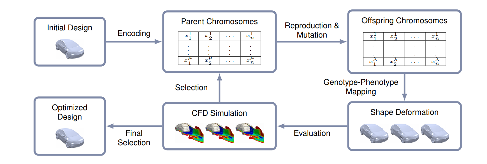
# What is evolutionary optimization?
## 1 1
~~~
$t := 0$;
initialize $P(0) := \{\vec{a}_1(0),\dots,\vec{a}_\mu(0)\} \in I^\mu$;
evaluate $F(0) : \{\Phi(x) | x \in P(0)\}$;
while($c(F(t)) \neq$ true) {
recombine: $P’(t) := r(P(t))$;
mutate: $P''(t) := m(P’(t))$;
evaluate $F(t) : \{\Phi(x) | x \in P''(t)\}$
select: $P(t + 1) := s(P''(t) \cup Q,\Phi)$;
$t := t + 1$;
}
~~~
~~~
$t$: Iteration-step
$I$: Set of possible Individuals
$P$: Population of Individuals
$F$: Fitness of Individuals
$Q$: Either set of parents or $\emptyset$
$r(..) : I^\mu \mapsto I^\lambda$
$m(..) : I^\lambda \mapsto I^\lambda$
$s(..) : I^{\lambda + \mu} \mapsto I^\mu$
~~~
- Algorithm to model simple inheritance
- Consists of three main steps
- recombination
- mutation
- selection
- An "individual" in our case is the displacement of control-points
# Evolutional loop
- **Recombination** generates $\lambda$ new individuals based on the characteristics of the $\mu$ parents.
- This makes sure that the next guess is close to the old guess.
- **Mutation** introduces new effects that cannot be produced by mere recombination of the
parents.
- Typically these are minor defects to individual members of the population
i.e. through added noise
- **Selection** selects $\mu$ individuals from the children (and optionally the
parents) using a *fitness--function* $\Phi$.
- Fitness could mean low error, good improvement, etc.
- Fitness not solely determines who survives, there are many possibilities
# Outline
- What is FFD?
- What is evolutionary optimization?
- **How to measure evolvability?**
- Scenarios
- Results
# How to measure evolvability?
- Different (conflicting) optimization targets
- convergence speed?
- convergence quality?
- As $\vec{v} = \vec{U}\vec{p}$ is linear, we can also look at $\Delta \vec{v} = \vec{U}\,
\Delta \vec{p}$
- We only change $\Delta \vec{p}$, so evolvability should only use $\vec{U}$
for predictions
# Evolvability criteria
- **Variability**
- roughly: "How many actual Degrees of Freedom exist?"
- Defined by
$$\mathrm{variability}(\vec{U}) := \frac{\mathrm{rank}(\vec{U})}{n} \in [0..1]$$
- in FFD this is $1/\#\textrm{CP}$ for the number of control-points used for
parametrization
# Evolvability criteria
- **Regularity**
- roughly: "How numerically stable is the optimization?"
- Defined by
$$\mathrm{regularity}(\vec{U}) := \frac{1}{\kappa(\vec{U})} = \frac{\sigma_{min}}{\sigma_{max}} \in [0..1]$$
with $\sigma_{min/max}$ being the least/greatest right singular value.
- high, when $\|\vec{Up}\| \propto \|\vec{p}\|$
# Evolvability criteria
- **Improvement Potential**
- roughly: "How good can the best fit become?"
- Defined by
$$\mathrm{potential}(\vec{U}) := 1 - \|(\vec{1} - \vec{UU}^+)\vec{G}\|^2_F$$
with a unit-normed guessed gradient $\vec{G}$
# Outline
- What is FFD?
- What is evolutionary optimization?
- How to measure evolvability?
- **Scenarios**
- Results
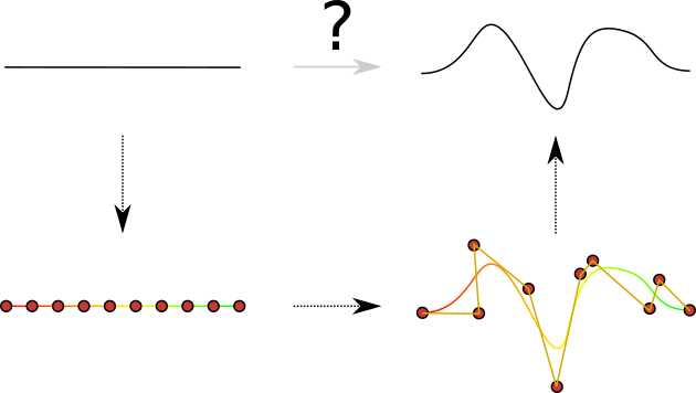
# Scenarios
- 2 Testing Scenarios
- 1-dimensional fit
- $xy$-plane to $xyz$-model, where only the $z$-coordinate changes
- can be solved analytically with known global optimum
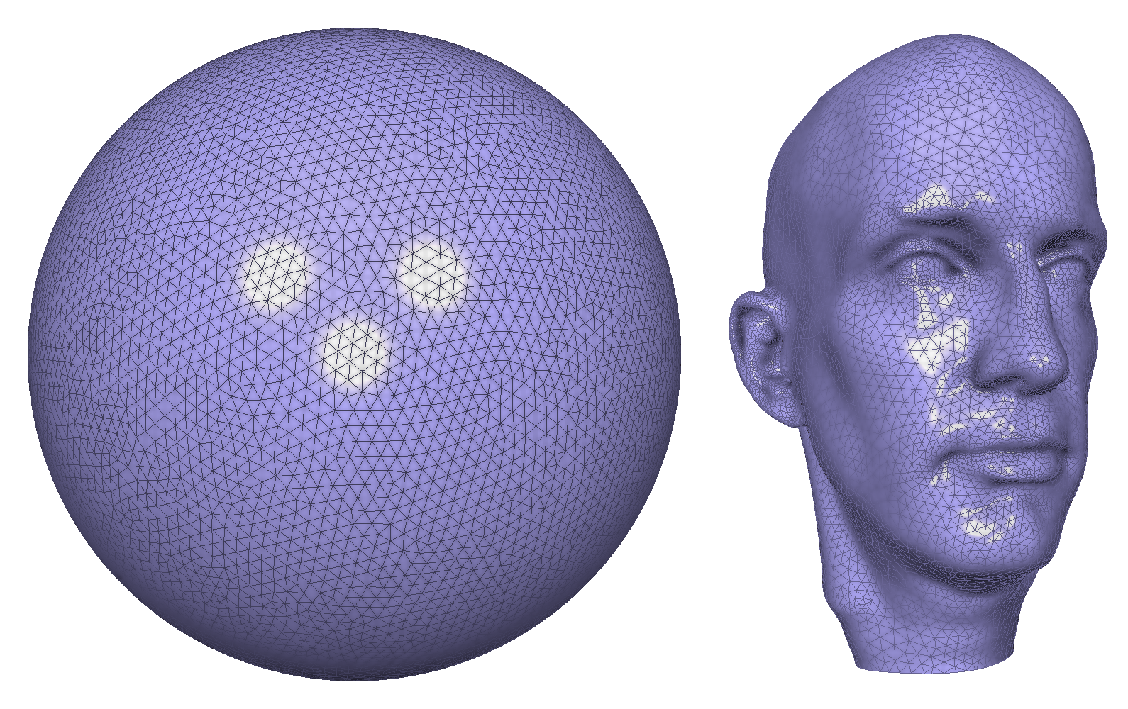
- 3-dimensional fit
- fit a parametrized sphere into a face
- cannot be solved analytically
- number of vertices differ between models
# 1D-Scenario
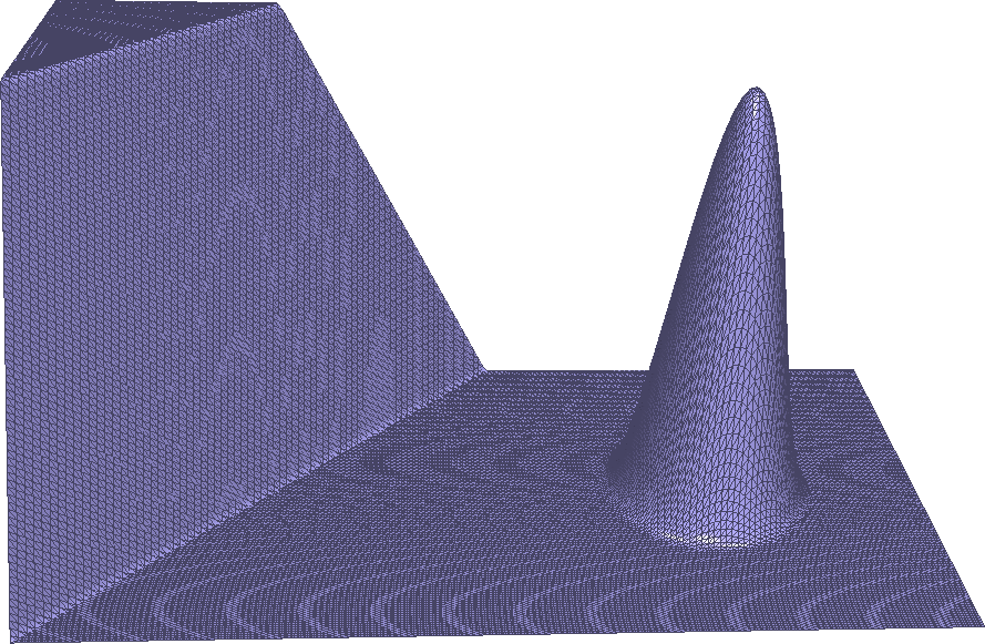{width=70%}
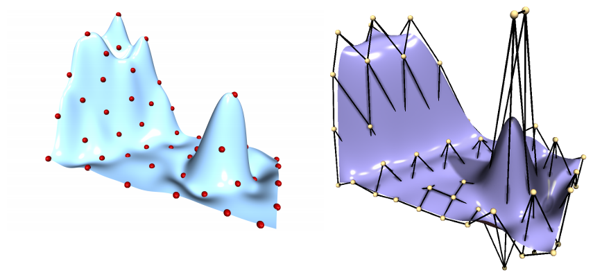
# 3D-Scenarios
# Outline
- What is FFD?
- What is evolutionary optimization?
- How to measure evolvability?
- Scenarios
- **Results**
# Variability 1D
- Should measure Degrees of Freedom and thus quality

- $5 \times 5$, $7 \times 7$ and $10 \times 10$ have *very strong* correlation ($-r_S = 0.94, p = 0$) between the *variability* and the evolutionary error.
# Variability 3D
- Should measure Degrees of Freedom and thus quality

- $4 \times 4 \times 4$, $5 \times 5 \times 5$ and $6 \times 6 \times 6$ have *very strong* correlation ($-r_S = 0.91, p = 0$) between the *variability* and the evolutionary error.
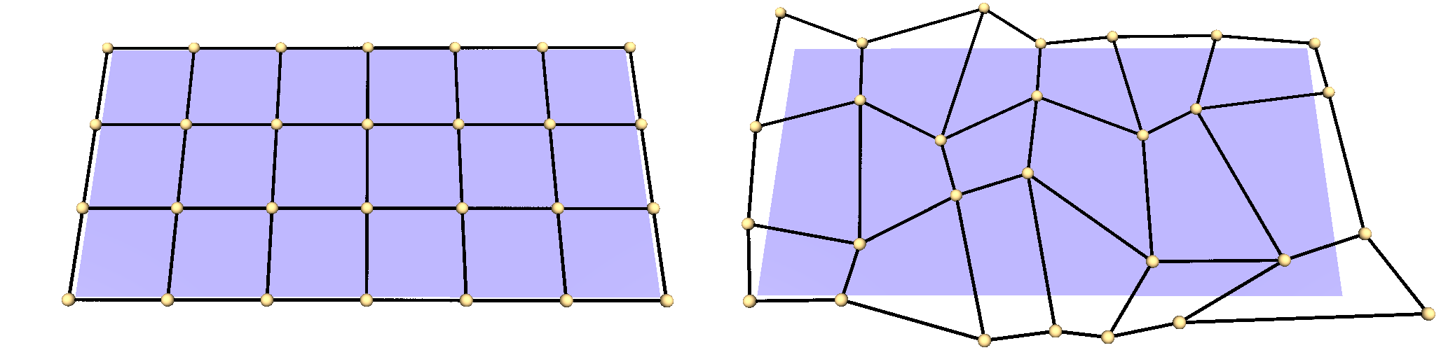
# Varying Variability
## 1 1

# Regularity 1D
- Should measure convergence speed
{width=70%}
- Not in our scenarios - maybe due to the fact that a better solution simply
takes longer to converge, thus dominating.
# Regularity 3D
- Should measure convergence speed
{width=70%}
- Only *very weak* correlation
- Point that contributes the worst dominates regularity by lowering the least
right singular value towards 0.
# Improvement Potential in 1D
- Should measure expected quality given a gradient
{width=70%}
- *very strong* correlation of $- r_S = 1.0, p = 0$.
- Even with a distorted gradient
# Improvement Potential in 3D
- Should measure expected quality given a gradient
{width=70%}
- *weak* to *moderate* correlation within each group.
# Summary
- *Variability* and *Improvement Potential* are good measurements in our cases
- *Regularity* does not work well because of small singular right values
- But optimizing for regularity *could* still lead to a better grid-setup
(not shown, but likely)
- Effect can be dominated by other factors (i.e. better solutions just take
longer)
# Outlook / Further research
- Only focused on FFD, but will DM-FFD perform better?
- for RBF the indirect manipulation also performed worse than the direct one
- Do grids with high regularity indeed perform better?
# Thank you
Any questions?