Evaluation of the Performance of Randomized FFD Control Grids
Master Thesis
Stefan Dresselhaus
Graphics & Geometry Group
Introduction
Many modern industrial design processes require advanced optimization methods due to increased complexity
Examples are
physical domains
aerodynamics (i.e. drag)
fluid dynamics (i.e. throughput of liquid)
NP-hard problems
layouting of circuit boards
stacking of 3D–objects
Motivation
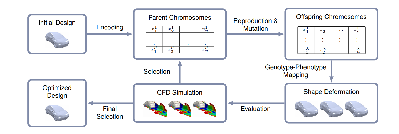
Evolutionary algorithms cope especially well with these problem domains Example of the use of evolutionary algorithms in automotive design
But formulation can be tricky
Motivation
Problems tend to be very complex
i.e. a surface with \(n\) vertices has \(3\cdot n\) Degrees of Freedom (DoF).
Need for a small-dimensional representation that manipulates the high-dimensional problem-space.
We concentrate on smooth deformations (\(C^3\)-continuous)
But what representation is good?
What representation is good?
In biological evolution this measure is called evolvability.
no consensus on definition
meaning varies from context to context
measurable?
Measure depends on representation as well.
RBF and FFD
Andreas Richter uses Radial Basis Functions (RBF) to smoothly deform meshes
Example of RBF–based deformation and FFD targeting the same mesh.
RBF and FFD
My master thesis transferred his idea to Freeform-Deformation (FFD)
same setup
same measurements
same results?
Example of RBF–based deformation and FFD targeting the same mesh.
Outline
What is FFD?
What is evolutionary optimization?
How to measure evolvability?
Scenarios
Results
What is FFD?
Create a function \(s : [0,1[^d \mapsto \mathbb{R}^d\) that is parametrized by some special control–points \(p_i\) with coefficient functions \(a_i(u)\): \[
s(\vec{u}) = \sum_i a_i(\vec{u}) \vec{p_i}
\]
All points inside the convex hull of \(\vec{p_i}\) accessed by the right \(u \in [0,1[^d\).
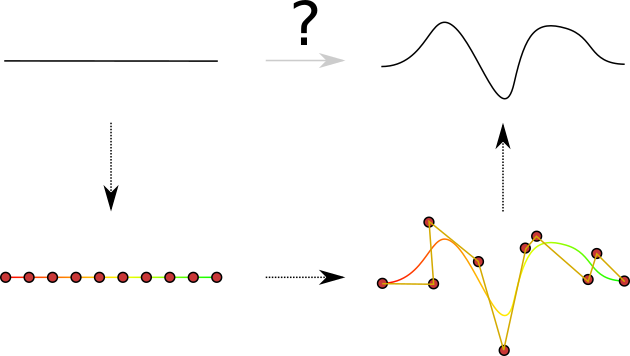
Example of a parametrization of a line with corresponding deformation to generate a deformed objet
Definition B-Splines
The coefficient functions \(a_i(u)\) in \(s(\vec{u}) = \sum_i a_i(\vec{u}) \vec{p_i}\) are different for each control-point
Given a degree \(d\) and position \(\tau_i\) for the \(i\)th control-point \(p_i\) we define \[\begin{equation}
N_{i,0,\tau}(u) = \begin{cases} 1, & u \in [\tau_i, \tau_{i+1}[ \\ 0, & \mbox{otherwise} \end{cases}
\end{equation}\] and \[\begin{equation} \label{eqn:ffd1d2}
N_{i,d,\tau}(u) = \frac{u-\tau_i}{\tau_{i+d}} N_{i,d-1,\tau}(u) + \frac{\tau_{i+d+1} - u}{\tau_{i+d+1}-\tau_{i+1}} N_{i+1,d-1,\tau}(u)
\end{equation}\]
The derivatives of these coefficients are also easy to compute: \[\frac{\partial}{\partial u} N_{i,d,r}(u) = \frac{d}{\tau_{i+d} - \tau_i} N_{i,d-1,\tau}(u) - \frac{d}{\tau_{i+d+1} - \tau_{i+1}} N_{i+1,d-1,\tau}(u)\]
Properties of B-Splines
Coefficients vanish after \(d\) differentiations
Coefficients are continuous with respect to \(u\)
A change in prototypes only deforms the mapping locally
(between \(p_i\) to \(p_{i+d+1}\))
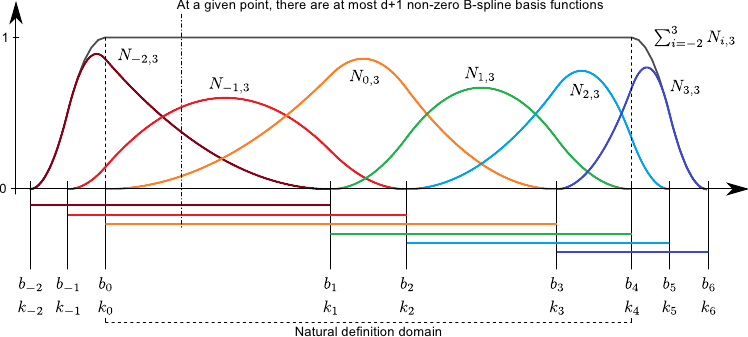
Example of Basis-Functions for degree \(2\). [Brunet, 2010] Note, that Brunet starts his index at \(-d\) opposed to our definition, where we start at \(0\).
Definition FFD
FFD is a space-deformation resulting based on the underlying B-Splines
Coefficients of space-mapping \(s(u) = \sum_j a_j(u) p_j\) for an initial vertex \(v_i\) are constant
Set \(u_{i,j}~:=~N_{j,d,\tau}\) for each \(v_i\) and \(p_j\) to get the projection: \[
v_i = \sum_j u_{i,j} \cdot p_j = \vec{u}_i^{T} \vec{p}
\] or written with matrices: \[
\vec{v} = \vec{U} \vec{p}
\]
\(\vec{U}\) is called deformation matrix
Implementation of FFD
As we deal with 3D-Models we have to extend the introduced 1D-version
We get one parameter for each dimension: \(u,v,w\) instead of \(u\)
Task: Find correct \(u,v,w\) for each vertex in our model
We used a gradient-descent (via the gauss-newton algorithm)
Implementation of FFD
Given \(n,m,o\) control-points in \(x,y,z\)–direction each Point inside the convex hull is defined by \[V(u,v,w) = \sum_i \sum_j \sum_k N_{i,d,\tau_i}(u) N_{j,d,\tau_j}(v) N_{k,d,\tau_k}(w) \cdot C_{ijk}.\]
Given a target vertex \(\vec{p}^*\) and an initial guess \(\vec{p}=V(u,v,w)\) we define the error–function for the gradient–descent as: \[Err(u,v,w,\vec{p}^{*}) = \vec{p}^{*} - V(u,v,w)\]
Armed with this we iterate the formula \[J(Err(u,v,w)) \cdot \Delta \left( \begin{array}{c} u \\ v \\ w \end{array} \right) = -Err(u,v,w)\] using Cramer’s rule for inverting the small Jacobian.
Usually terminates after \(3\) to \(5\) iteration with an \(\epsilon := \vec{p^*} - V(u,v,w) < 10^{-4}\)
self-intersecting grids can invalidate the results
no problem, as these get not generated and contradict some properties we want (like locality)
$t$: Iteration-step
$I$: Set of possible Individuals
$P$: Population of Individuals
$F$: Fitness of Individuals
$Q$: Either set of parents or $\emptyset$

$r(..) : I^\mu \mapsto I^\lambda$
$m(..) : I^\lambda \mapsto I^\lambda$
$s(..) : I^{\lambda + \mu} \mapsto I^\mu$
Algorithm to model simple inheritance
Consists of three main steps
recombination
mutation
selection
An “individual” in our case is the displacement of control-points
Evolutional loop
Recombination generates \(\lambda\) new individuals based on the characteristics of the \(\mu\) parents.
This makes sure that the next guess is close to the old guess.
Mutation introduces new effects that cannot be produced by mere recombination of the parents.
Typically these are minor defects to individual members of the population i.e. through added noise
Selection selects \(\mu\) individuals from the children (and optionally the parents) using a fitness–function\(\Phi\).
Fitness could mean low error, good improvement, etc.
Fitness not solely determines who survives, there are many possibilities
Outline
What is FFD?
What is evolutionary optimization?
How to measure evolvability?
Scenarios
Results
How to measure evolvability?
Different (conflicting) optimization targets
convergence speed?
convergence quality?
As \(\vec{v} = \vec{U}\vec{p}\) is linear, we can also look at \(\Delta \vec{v} = \vec{U}\, \Delta \vec{p}\)
We only change \(\Delta \vec{p}\), so evolvability should only use \(\vec{U}\) for predictions
Evolvability criteria
Variability
roughly: “How many actual Degrees of Freedom exist?”
Defined by \[\mathrm{variability}(\vec{U}) := \frac{\mathrm{rank}(\vec{U})}{n} \in [0..1]\]
in FFD this is \(1/\#\textrm{CP}\) for the number of control-points used for parametrization
Evolvability criteria
Regularity
roughly: “How numerically stable is the optimization?”
Defined by \[\mathrm{regularity}(\vec{U}) := \frac{1}{\kappa(\vec{U})} = \frac{\sigma_{min}}{\sigma_{max}} \in [0..1]\] with \(\sigma_{min/max}\) being the least/greatest right singular value.
high, when \(\|\vec{Up}\| \propto \|\vec{p}\|\)
Evolvability criteria
Improvement Potential
roughly: “How good can the best fit become?”
Defined by \[\mathrm{potential}(\vec{U}) := 1 - \|(\vec{1} - \vec{UU}^+)\vec{G}\|^2_F\] with a unit-normed guessed gradient \(\vec{G}\)
Outline
What is FFD?
What is evolutionary optimization?
How to measure evolvability?
Scenarios
Results
Scenarios
2 Testing Scenarios
1-dimensional fit
\(xy\)-plane to \(xyz\)-model, where only the \(z\)-coordinate changes
can be solved analytically with known global optimum
3-dimensional fit
fit a parametrized sphere into a face
cannot be solved analytically
number of vertices differ between models
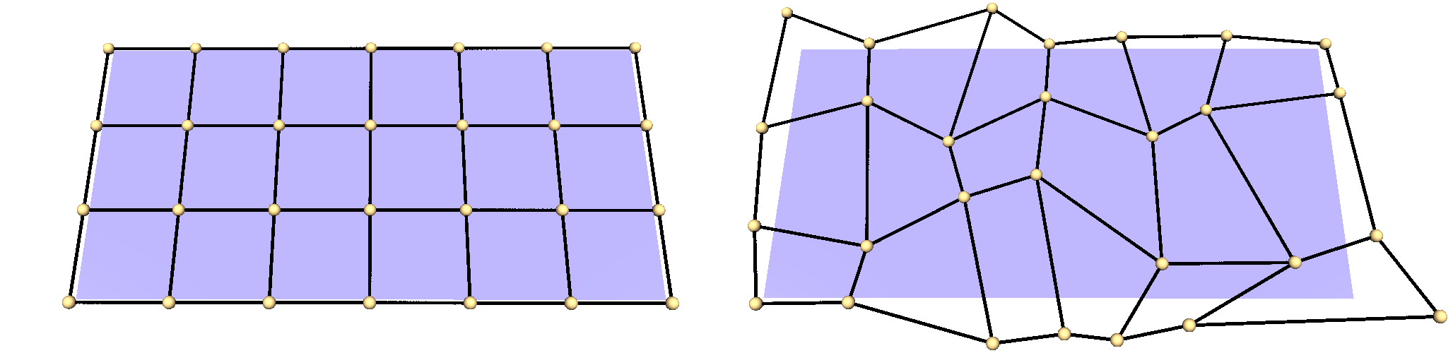
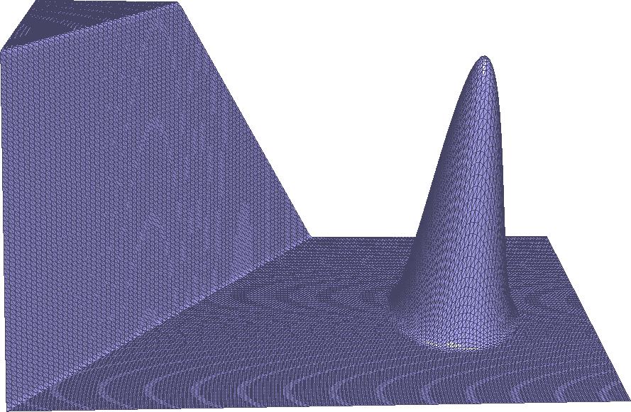
1D-Scenario
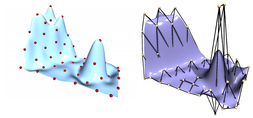
Left: A regular \(7 \times 4\)–grid Right: The same grid after a random distortion to generate a testcase.
The target–shape for our 1–dimensional optimization–scenario including a wireframe–overlay of the vertices.
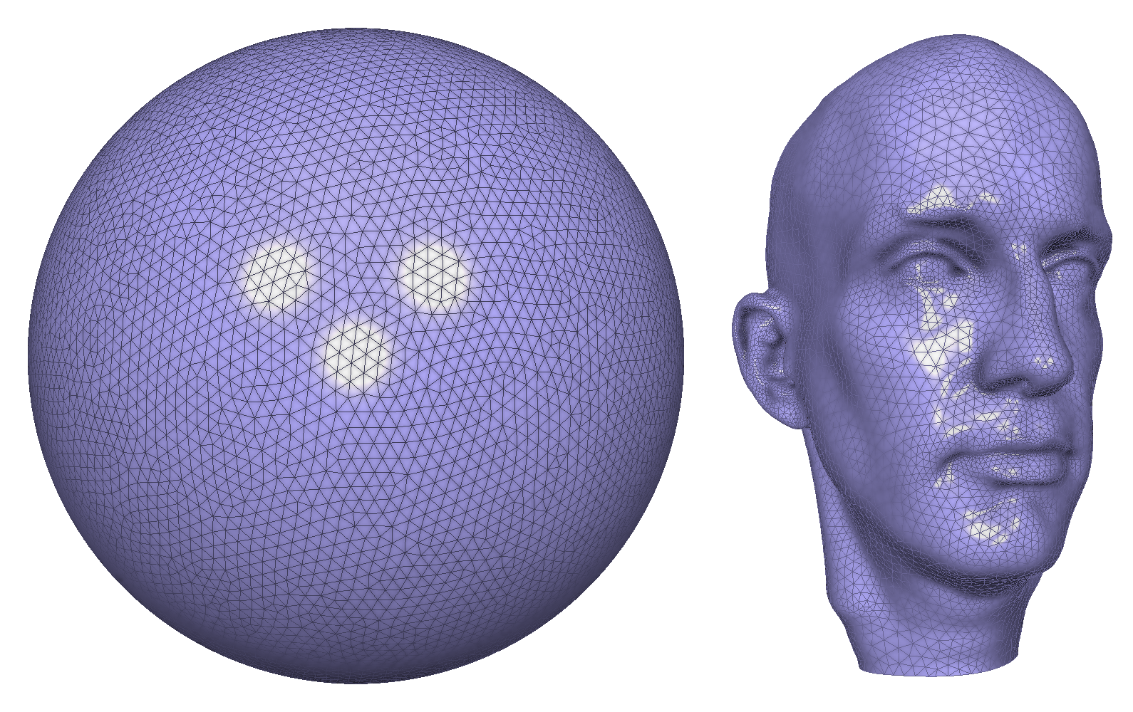
3D-Scenarios
Left: The sphere we start from with 10 807 vertices Right: The face we want to deform the sphere into with 12 024 vertices.
Outline
What is FFD?
What is evolutionary optimization?
How to measure evolvability?
Scenarios
Results
Variability 1D
Should measure Degrees of Freedom and thus quality
The squared error for the various grids we examined. Note that \(7 \times 4\) and \(4 \times 7\) have the same number of control–points.
\(5 \times 5\), \(7 \times 7\) and \(10 \times 10\) have very strong correlation (\(-r_S = 0.94, p = 0\)) between the variability and the evolutionary error.
Variability 3D
Should measure Degrees of Freedom and thus quality
The fitting error for the various grids we examined. Note that the number of control–points is a product of the resolution, so \(X \times 4 \times 4\) and \(4 \times 4 \times X\) have the same number of control–points.
\(4 \times 4 \times 4\), \(5 \times 5 \times 5\) and \(6 \times 6 \times 6\) have very strong correlation (\(-r_S = 0.91, p = 0\)) between the variability and the evolutionary error.
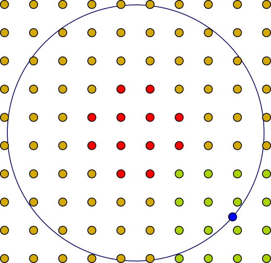
Varying Variability
A high resolution (\(10 \times 10\)) of control–points over a circle. Yellow/green points contribute to the parametrization, red points don’t. An Example–point (blue) is solely determined by the position of the green control–points.
Histogram of ranks of various \(10 \times 10 \times 10\) grids with \(1000\) control–points each showing in this case how many control–points are actually used in the calculations.
Regularity 1D
Should measure convergence speed
Left: Improvement potential against number of iterations until convergence Right: Regularity against number of iterations until convergence Coloured by their grid–resolution, both with a linear fit over the whole dataset.
Not in our scenarios - maybe due to the fact that a better solution simply takes longer to converge, thus dominating.
Regularity 3D
Should measure convergence speed
Plots of regularity against number of iterations for various scenarios together with a linear fit to indicate trends.
Only very weak correlation
Point that contributes the worst dominates regularity by lowering the least right singular value towards 0.
Improvement Potential in 1D
Should measure expected quality given a gradient
Improvement potential plotted against the error yielded by the evolutionary optimization for different grid–resolutions
very strong correlation of \(- r_S = 1.0, p = 0\).
Even with a distorted gradient
Improvement Potential in 3D
Should measure expected quality given a gradient
Plots of improvement potential against error given by our fitness–function after convergence together with a linear fit of each of the plotted data to indicate trends.
weak to moderate correlation within each group.
Summary
Variability and Improvement Potential are good measurements in our cases
Regularity does not work well because of small singular right values
But optimizing for regularity could still lead to a better grid-setup (not shown, but likely)
Effect can be dominated by other factors (i.e. better solutions just take longer)
Outlook / Further research
Only focused on FFD, but will DM-FFD perform better?
for RBF the indirect manipulation also performed worse than the direct one
Do grids with high regularity indeed perform better?